Data Visualization: 200 Years of Health and Wealth

This video is super awesome!  It's part of BBC 4's program The Joy of Stats and you can learn a little more about the data here or play with it using this web app on http://www.gapminder.org/. Now don't you wish you could do that with data?

The reason I wanted to share this video (beyond the fact that it's so amazingly awesome) is to let you in on a little secret... are you ready? Here it comes...

Data visualization is easy, and anyone with a computer can do it!

Seriously, it is not that hard! YOU can make cool little wobbling bubble graphs just like in the video! Aren't you excited to learn how?! Yeah? Fantastic!

Now that you're all psyched to visualize some data, I should mention that I am being a bit misleading here... because it does require a bit of computer know-how, and sometimes (ok, almost always) takes a bit of tinkering with the data to find the best ways of boiling down to just the relevant information. But frankly, these things aren't all that hard to learn and aren't always necessary if we're just poking around to get a feel for the data, so none of these words of caution should give you much pause.  Add to that the fact you can always hit up the internet for examples to download and use study and learn from and many of these obstacles are reduced to mere speed bumps.  If you've got a computer, we can get it to plot some data.

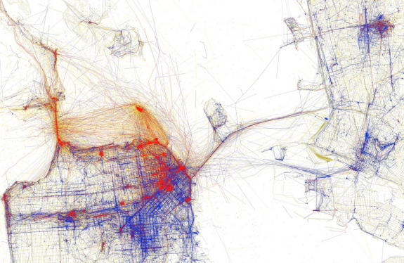
Figure 1. Tourist hot spots based on Flickr data. #1 of flowingdata's Top Ten Data Visualization Projects of 2010.

So here's the deal... there are some really cool data available from http://www.gapminder.org/, and I'm going to have a little free time these next few weeks in between birding trips, visiting family and friends, and doing thesis work.  Assuming that free time stays free, I'm going to walk through an example or two of plotting some of this data in R.  If you'd like to follow along, you'll need to download and install R on your computer, and if you don't already have software that can open excel spreadsheets, you'll also want to install something (free) like OpenOffice.

Sound good? Excellent!  Feel free to share any questions or suggestions in the comments section below.  Now hurry along and go install R!

Support Wildlife Conservation in Ohio

Buy an Ohio Wildlife Legacy stamp!

While hunters automatically contribute funds towards the conservation coffers each time they purchase a hunting licenses, wildlife watchers (like birders and herpers) and native plant aficionados aren't required to make such contributions when they go outside to enjoy their favorite organisms. The result? Less money for habitat and wildlife conservation.

The Ohio Wildlife Legacy stamps are an attempt to fix this problem, by inviting all those non-hunters to contribute. With the holidays coming up, and at only $15 each, they make great gifts for that outdoorsy guy or gal on your gift list.  Even for those who do hunt or fish, and already buy licenses (which I believe can't be purchased as a gift) the Wildlife Legacy stamp might still be a much appreciated gift.

To purchase one (or more!), you can buy them online from the ODNR website, the Columbus Audubon Society's website, or you can buy them in person at the nearest ODNR Wildlife District Office.

Knotty Doodles

Fast and Sloppy Root Finding

Disclaimer: While the approach to root finding mentioned below is both slow and imprecise, it's also a cheap and incredibly handy approach when all you need to do is get "close enough". If you like R quick and dirty (hey now, get your mind out of the gutter...) this is totally the root finding method for you!

I just read a post on Root Finding (original here) by way of R-bloggers.com which was timely given that only yesterday I'd needed to do some root finding in R to make a figure for a manuscript -- something like the following image.

The blog post prompted me to mention here how I did my root finding for two reasons:

1. Precision and computation time sometimes don't matter all that much; and
2. The way I did my root finding was way easier to implement than convergence-based methods described in the post above.

So here's what I was aiming for, and how I implemented it in R.

The Task: Suppose you're plotting two curves (say, y=f(x) and y=g(x)) and would like to indicate their intersection with an empty circle (i.e. pch=21). In my case, the intersection of these two curves was equilibrium point for a dynamic model, and I wanted to indicate it as such.

If you can find their intersection mathematically (i.e. set f(x)=g(x) and solve for x) then awesome -- do that if you can.  But if for some reason you can't, and you know a single root exists in some interval a≤x≤b, you can find that root quickly using some straightforward vector tricks.

The Solution: Lets use the example of finding the intersection of f(x) = x/(1+x) and g(x) = (5-x)/5 over the interval (0,5).

Step 1:  Define an x vector full of values between a and b.  The smaller the step size (or, the longer the list) the better.

> x = seq(0, 5, length=5000);

Step 2: Compute the square of the difference of your two functions over that interval using x.  This is as simple as the line of code...

> fgdiff = ( x/(1+x) - (5-x)/5 )^2;

Step 3: Using the which() function, we can pick out the index for the smallest value in our list of squared differences... Once we know this index (call it j) we know the intersection occurs at, or very near, the x value x[j], and we're basically done! 

> j = which(fgdiff==min(fgdiff))[1]; 
> j; x[j];  ## show the value of j, x[j]

For a closer look at what's going on with that which() statement, check out the help for which() and following example.

## A Closer look at the which(fgdiff==min(fgdiff))
> ?which
> which(c(F,F,T,T,F))
[1] 3 4
> which(c(F,F,T,T,F))[1]
[1] 3
> xample = c(5:1,2:5); xample
[1] 5 4 3 2 1 2 3 4 5
> min(xample)
[1] 1
> xample==min(xample)
[1] FALSE FALSE FALSE FALSE  TRUE FALSE FALSE FALSE FALSE
> which(xample==min(xample))
[1] 5
> which(xample==min(xample))[1]
[1] 5

Step 4: Since both functions are (approximately) equal at this x value, it only remains to decide whether you want to indicate the point of intersection using (x, f(x)) or (x, g(x)).

> points(x[j], x[j]/(1+x[j]), pch=19, cex=2)

All done!

If you'd like to tinker with this example, here's the code to produce the image above.